Data Processing, Alignment, and Segmentation

Data Deluge and the Processing Pipeline

The advent of volume electron microscopy (vEM), and specifically Serial Block-Face Scanning Electron Microscopy (SBF-SEM), has propelled biological ultrastructural analysis firmly into the "big data" paradigm [168]. A single high-resolution SBF-SEM instrument can easily generate over 250 gigabytes of image data per day, and comprehensive volumetric tissue studies frequently accrue massive datasets scaling into the hundreds of terabytes [16], [168]. Consequently, while historical limitations in electron microscopy were largely constrained by primary data acquisition and manual sectioning, the primary bottleneck has decisively shifted downstream. The challenge now lies in the computational management, post-processing, and semantic interpretation of these massive datasets [14], [14], [35], [17], [19]. Transforming a vast collection of raw backscattered electron micrographs into a biologically interpretable, geometrically accurate three-dimensional volume requires a sequential and highly robust data processing workflow [14], [19], [19], [19], [19], [9], [19]. This downstream pipeline fundamentally consists of raw data pre-processing, image enhancement, stack alignment and registration, feature segmentation, volumetric reconstruction, and ultimately, quantitative spatial analysis [14], [26], [18], [18], [19], [166] (Figures 21–23).

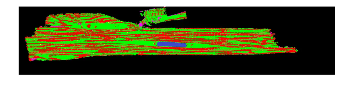
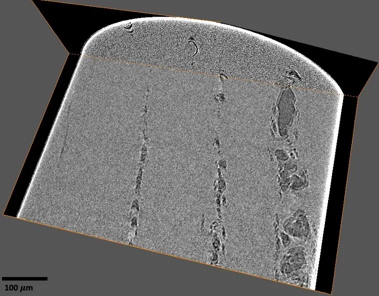
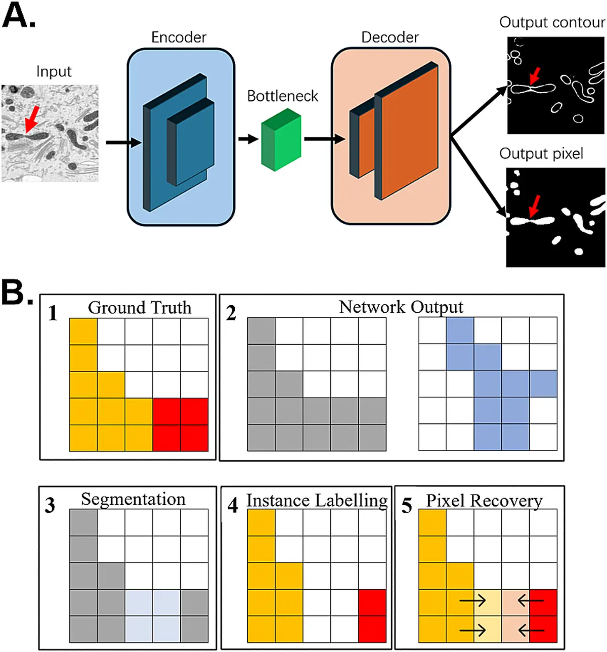
Image Pre-Processing, Enhancement, and Noise Reduction

Raw SBF-SEM datasets are generally acquired as proprietary digital formats, such as Gatan’s Digital Micrograph (.dm3 or .dm4) files [17], [26], [81], [18], [156]. The foundational step in data processing involves the conversion of these proprietary files into universally accessible 8-bit or 32-bit TIFF or MRC image sequences [17], [26], [111], [81], [18], [156], [17]. Because raw images are frequently captured at a 16-bit depth, systematically converting them to an 8-bit format is a standard practice used to significantly reduce the overall file size and ease subsequent computational processing loads without sacrificing biologically relevant contrast [28], [111], [81], [156], [81]. Furthermore, due to the vastness of the fields of view, image stacks are frequently downsampled or cropped to specific regions of interest (ROIs). This targeted cropping systematically eliminates unnecessary background spaces, mitigates empty edge artefacts generated by rotational alignments, and minimises the data footprint prior to intensive algorithmic processing [84], [152], [111], [143], [84], [143].

Image enhancement is essential to correct for inherent imaging artefacts and to standardise image quality throughout the Z-stack. Normalisation of brightness and contrast is universally applied to counteract varying backscattered electron signal intensities or slight charging artefacts that manifest across consecutive slices [9], [84], [150], [81], [18], [156], [150], [166]. Techniques such as contrast-limited adaptive histogram equalisation (CLAHE) are frequently employed to improve local contrast within small cellular regions without unduly amplifying background noise [143]. More precise techniques, such as exact histogram specification, mathematically match the histogram of every sequential slice to that of a reference image (often the first slice), ensuring strict grayscale consistency throughout the reconstructed volume [150], [150]. Additionally, SBF-SEM imaging often suffers from elevated noise levels owing to the very short pixel dwell times (often 1–3 µs) required to prevent excessive beam damage to the resin block [28], [145], [59], [49], [55], [84]. To mitigate this noise, smoothing filters such as Gaussian blurs, median filters, and band-pass filters are routinely applied to increase the signal-to-noise ratio prior to segmentation [84], [150], [152], [81], [156], [127], [49], [84], [160], [50].

Recently, computational deconvolution techniques—traditionally a staple of light microscopy—have been adapted for volume EM. By mathematically modelling the 3D SBF-SEM point spread function (PSF) via Monte Carlo simulations of electron scattering within the resin, researchers can deconvolve the image stacks. This advanced approach significantly recovers structural detail, reduces high-frequency noise, and computationally enhances the typically anisotropic Z-resolution of SBF-SEM data [145], [32], [145], [32], [42].

Image Alignment and Stack Registration

SBF-SEM benefits from an inherent physical advantage over serial section transmission electron microscopy (ssTEM) or array tomography: because images are acquired sequentially from a rigid, stationary block face within the microscope vacuum chamber, they are fundamentally in register [48], [147], [26], [12], [59], [34], [81], [86], [29], [12], [16], [14], [97], [14]. The technique avoids the gross mechanical distortions, section losses, or rotational warping seen in traditional ultra-microtomy collection methods. Nevertheless, raw SBF-SEM alignment is almost never perfect. Subtle misalignments, image jitter, and spatial drift regularly occur due to thermal fluctuations, mechanical stage instabilities, and local deflections of the electron beam caused by the build-up of electrostatic surface charge [14], [14], [28], [147], [13], [20], [86], [111], [86], [147], [28], [55]. Restoring single-pixel precision continuity through the Z-stack is therefore crucial, particularly when preparing data for automated segmentation algorithms and 3D rendering [14], [147], [13], [20], [147].

Fine alignment workflows typically employ cross-correlation techniques [9], [147], [150], [86], [86], [147] or feature-matching algorithms, most notably the Scale-Invariant Feature Transform (SIFT) [9], [28], [20], [86], [111], [81], [86], [147], [28], [159], [147], [5], [143]. Open-source software environments like Fiji/ImageJ are routinely used to execute these alignments via plugins such as "Register Virtual Stack Slices" or "Linear Stack Alignment with SIFT" [148], [151], [86], [111], [86], [156], [49], [55], [143]. Crucially, standard SBF-SEM alignment generally restricts transformations to rigid translation (x and y planar shifts) while specifically prohibiting affine scaling, elastic warping, or rotation. Stack alignment methods that manipulate image data by arbitrary deformation are generally undesirable, as they risk artificially warping the true biological morphology and introducing geometrical inaccuracies [14], [14], [28], [148], [151], [86], [111], [86], [28].

However, for particularly large datasets requiring the correction of complex local distortions, or for mosaic stitching of multiple overlapping tiles per slice, advanced software suites such as TrakEM2 [9], [59], [20], [16], [164], [166], IMOD [20], [147], [16], [3], Microscopy Image Browser (MIB) [16], and TeraStitcher [20], [147] are employed. TrakEM2, for example, expands upon the SIFT concept to globally minimise registration errors and algorithmically correct lens distortions across vast fields of view [9], [16], [166]. Advanced non-rigid alignment methods have also been carefully explored to correct for specific charging artefacts; these include "as-rigid-as-possible" alignment protocols [14], [14] and optical flow-based "Demon" registration algorithms. Demon registration utilises multi-scale grid spacings to cope with local geometric warping induced by charging, while penalising extreme global image deformation, thereby finding a compromise between accurate registration and smooth transformation fields [13], [17], [97].

The Segmentation Bottleneck: Manual and Semi-Automated Approaches

Once an SBF-SEM stack is perfectly aligned and contrast-normalised, the data must be segmented. Segmentation is the intricate process of partitioning an image stack by assigning distinct voxels to specific biological objects, features, or organelles [48], [18], [18], [20], [12]. Despite immense algorithmic advances, segmentation remains the most formidable and time-consuming bottleneck in the entire vEM pipeline [14], [14], [153]. Extracting meaningful biological insights—whether mapping complete neuronal connectomes or quantifying intracellular organelle distributions—demands exceptionally high-fidelity object delineation [20].

Manual segmentation, whereby an experienced biologist anatomically traces the outlines of features slice-by-slice, provides the highest degree of accuracy but is extraordinarily labour-intensive and excruciatingly slow [14], [48], [16], [18], [37], [18], [29], [32], [20], [16]. It has been estimated that it would take a single human up to 60 years of continuous work to manually segment every organelle within a single cell at high resolution [16]. To conquer the sheer volume of manual tracing required for complex neural circuits, crowdsourcing initiatives such as the Eyewire project—which employs citizen scientists via a computer game interface—or the use of Amazon Mechanical Turk have been leveraged [14], [37]. However, for the vast majority of laboratories, scaling up manual analysis is unfeasible, making the transition to software-assisted or fully automated pipelines an absolute necessity [14], [48], [16], [28], [32], [20], [168].

Semi-automated segmentation tools offer an intermediate step, combining human anatomical guidance with algorithmic prediction to rapidly accelerate the tracing process. A prominent technique is interpolation, where a user manually annotates a complex structure on every *n*th slice, and the software algorithmically predicts the morphological shape and automatically fills in the boundaries on the intervening slices [35], [155], [35], [20], [161], [35], [97], [35]. Additional semi-automated tools include region-growing algorithms, watershed segmentations that cluster pixels based on local intensity gradients, and "magic wand" tools that utilize polygon expansion over connected voxel contrast gradients [35], [35], [18], [18], [35], [20], [35], [97], [35], [151].

When biological samples are prepared with highly specific or aggressively contrasting heavy metal stains (e.g., lanthanum dysprosium for glycosaminoglycans, or ZIO for the Golgi apparatus), simple intensity-based thresholding can be applied [35], [28], [18], [154], [37], [18], [35], [20], [12], [35], [166], [97], [28], [12]. In these highly specific scenarios, users define a narrow grayscale value range, and the software automatically groups all correlating voxels into a defined object [20]. While computationally cheap, simple thresholding universally struggles with the complex, densely packed, and similarly electron-dense structures typical of standard *en bloc* stained SBF-SEM tissue samples. In complex neuropil or densely packed cellular environments, thresholding invariably fails to distinguish adjacent lipid membranes, necessitating massive amounts of manual error correction [48], [28].

Machine Learning and Deep Learning Segmentation Pipelines

To overcome the severe limitations of classical thresholding and semi-automated image analysis, machine learning (ML) and deep learning (DL) algorithms have increasingly dominated modern SBF-SEM segmentation workflows [48], [145], [149], [152], [18], [153], [39], [18], [32], [153], [149], [162], [149], [163], [165], [167], [117]. Early machine learning tools, such as the random forest classifiers implemented in the open-source software Ilastik, allow users to interactively train a pixel classifier by painting sparse, rapid labels onto the image, teaching the algorithm to distinguish between different textural classes [28], [153], [163].

More recently, deep Convolutional Neural Networks (CNNs) and deep learning architectures like U-Net have achieved state-of-the-art performance in vEM segmentation [153], [153], [163], [9]. In these advanced deep learning workflows, a very small subset (often less than 1%) of the image stack is manually annotated as "ground truth" to train the model [48], [153]. The trained network then autonomously predicts the segmentation for the entire volumetric dataset. Iterative training loops, where researchers visually inspect the output, correct the worst network predictions, and feed them back into the model, further enhance the accuracy and robustness of the segmentation [153].

Advanced deep learning tools like the Cascaded Hierarchical Model (CHM) [150], [150] and generalist deep-learning volume networks (such as the Volume Segmentation Tool (VST) or PyTorch Connectomics) are specifically designed to examine multi-slice volumetric data rather than processing stacks one 2D slice at a time [48], [149], [149], [149]. This multi-slice assessment provides crucial spatial continuity across the Z-axis that 2D networks inherently lack, mirroring the way a human anatomist flips back and forth between sections to identify complex morphological structures [149], [149], [149].

Furthermore, deep learning approaches are actively driving the analytical shift from simple *semantic segmentation* (predicting whether a pixel broadly belongs to a trained target class, such as "mitochondria") to *instance segmentation* (delineating separate, distinct objects of the same class, allowing the counting of individual mitochondria) [149], [149], [9]. Open-source tools such as Cellpose [162] and custom segmentation pipelines executed via CellProfiler [158] have demonstrated the profound capacity to perform accurate instance segmentation and object tracking across complex, densely packed tissue environments. Furthermore, transfer learning—the application of pre-trained neural networks to novel datasets—has been shown to massively improve performance and generalisability across diverse tissue types without requiring exhaustive new ground-truth annotations [162], [163].

3D Reconstruction and Visualisation

Following segmentation, the extracted binary masks and discrete object labels must be rendered into three-dimensional models. Visualisation is an indispensable component of SBF-SEM analysis, allowing researchers to accurately observe topological relationships, cell-to-cell arrangements, and intricate intracellular networks that are entirely impossible to discern from 2D orthoslices alone [14], [19], [32], [12], [18], [35], [39], [29], [22], [12], [149], [28]. Rendering software converts the segmented 3D voxel data into geometric mesh surface models (e.g., Boissonnat surfaces) or texture-based volume renders [19], [146], [18], [18], [17], [32].

A wide array of commercial and open-source software packages facilitate this structural reconstruction. Industry-standard software includes Amira (Thermo Fisher) [97], [59], [152], [35], [155], [37], [81], [18], [156], [49], [84], [32], [12], [12], [50], [35], [137], [97], [159], [12], Imaris (Bitplane) [37], Microscopy Image Browser (MIB) [59], [35], [28], [155], [81], [16], [35], 3DMOD/IMOD [20], [26], [59], [37], [81], [147], [150], [49], [20], [12], [16], [3], [12], ImageJ/Fiji [9], [59], [111], [81], [55], [12], [16], [35], [137], [17], ORS Dragonfly [19], [19], [19], [19], [19], [137], [19], [52], TESCAN 3D Analysis Suite [19], [19], [19], [19], [19], [19], [19], and Vaa3D [59], [81]. Frequently, researchers employ a combination of these platforms; for example, generating structural object files in Amira or Reconstruct, and subsequently exporting them as VRML or OBJ files for high-fidelity rendering, texturing, and dynamic animation in the open-source graphics suite Blender [146], [155], [35]. These visualisation tools empower researchers to virtually rotate tissues, generate digital cross-sections, and produce demonstrative animations that explore the ultrastructural depths of the datasets [146], [35], [155], [17], [50].

Quantitative Analysis and Data Management

Stunning 3D visualisation is rarely the final scientific endpoint; researchers must ultimately extract quantitative, morphometric data from the reconstructed models. This downstream analysis includes precise volumetric measurements, surface area calculations, absolute object counts, spatial distribution mapping, and complex calculations of structural tortuosity and branching [18], [18], [153], [154], [37], [18], [20], [137], [97], [173].

However, quantification requires careful geometrical consideration. SBF-SEM inherently yields highly anisotropic voxels. While the lateral (X and Y) resolution is dictated by the electron beam and may be as fine as 5–10 nanometres, the axial (Z) resolution is strictly determined by the physical cutting increment of the diamond knife, typically ranging from 25 to 100 nanometres [13], [32], [157], [32], [42], [137], [28], [32]. Volumetric measurements and automated deep learning models must mathematically account for this discrepancy [137]. For remarkably small or highly complex subcellular structures—such as the canalicular system in blood platelets—direct 3D volumetric counts may be skewed by the anisotropic Z-resolution, necessitating the application of classical stereological methods to ensure statistical accuracy [32], [32], [32]. Furthermore, substantial tissue shrinkage resulting from aggressive chemical fixation, dehydration, resin embedding, and intense electron beam exposure must be quantified. Correction factors must be mathematically applied to the 3D models to accurately reflect the true *in vivo* dimensions of the cellular components [151], [125], [166].

Finally, the vast scale and extreme computational expense of SBF-SEM output demand rigorous data management principles. Given the high cost of acquisition, vEM datasets possess immense secondary value. Image stacks and corresponding segmentation masks should ideally adhere to FAIR principles (Findability, Accessibility, Interoperability, and Reuse). These datasets must be accompanied by extensive metadata detailing the exact processing and segmentation workflow [17], [17], [35], [169]. Hosting raw and segmented terabyte-scale datasets in open-access repositories such as EMPIAR (Electron Microscopy Public Image Archive) or Nanotomy ensures profound reproducibility, prevents redundant resource expenditure, and provides invaluable ground-truth data essential for training the next generation of deep learning algorithms [62], [17], [35], [92], [169].