Case Studies

Six and a Half Days Without Charging: Precision Charge Neutralisation Across a 169-Gigavoxel Volume

ConnectomX Team·18 August 2026·14 min read

Precision Charge Neutralisation · Katana Microtome · Samurai 3 + TESCAN CLARA · Kensho BSED · Spod5, acquired 2026-08-03 → 2026-08-10

Abstract

Charging is the limiting factor when serial block-face imaging is applied to resin-embedded material. Over six and a half days, a Katana Microtome fitted with Precision Charge Neutralisation (PCN) cut and imaged the Spod5 specimen through 420 unattended cut-and-image cycles — 169 gigavoxels, 339 GB, 45.9 µm of sectioned depth at three nested scales down to 10 nm pixels — with the chamber at high vacuum the whole time. This report puts the charge-control evidence first: the gas field and its effect on charging, then the cut surface re-imaged in secondary electrons a day after the run. The volume that the neutralisation made possible, and the full acquisition record, follow.

Cycles completed

420

unattended cut-and-image

Acquisition duration

3.6 d

85 h of imaging

Chamber pressure

34 mPa

high vacuum, away from the needle

Sectioned depth

45.9 µm

70–100 nm sections

Voxels acquired

169.3 G

16-bit

Raw data

339 GB

uncompressed TIFF

Maximum electron dose

49.9

e⁻/nm² at 1.75 kV

Finest sampling

10 nm

8192² frames

Images acquired

7,292

across four ROIs

Throughput

30 min

per gigavoxel

Working distance

3.65 mm

main volumes

A non-conductive block face cannot shed the electrons the raster buries, so the field goes negative and bends the beam. Precision Charge Neutralisation answers that with a trace of gas delivered to the imaging site by a motorised needle and ionised by the beam itself, so the neutralisation is local and the chamber never leaves high vacuum. What follows is what that looked like across a full week-long acquisition.

1. The gas field

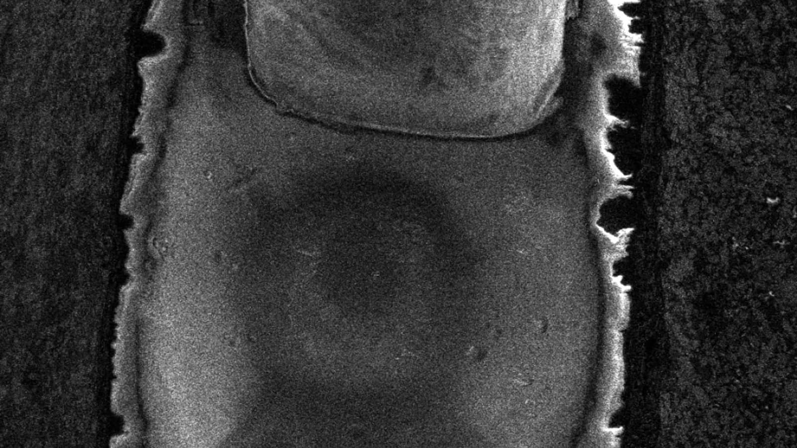
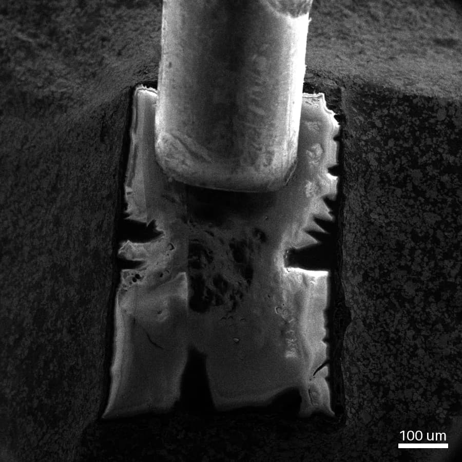
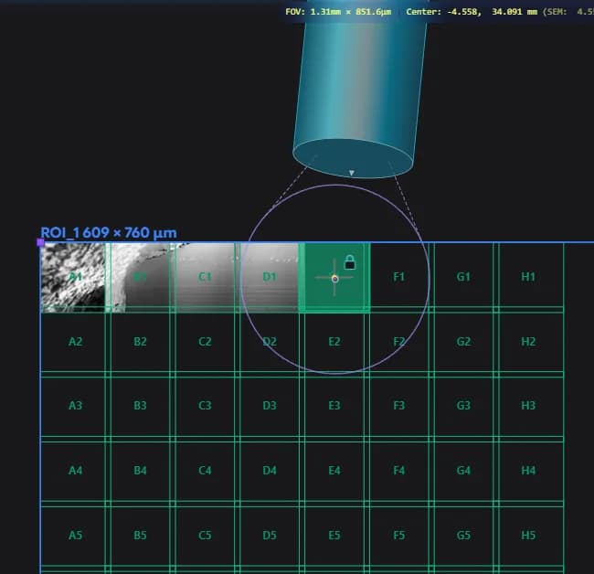
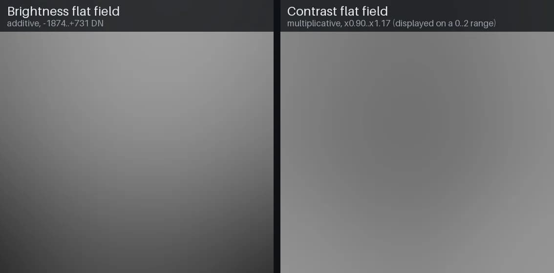
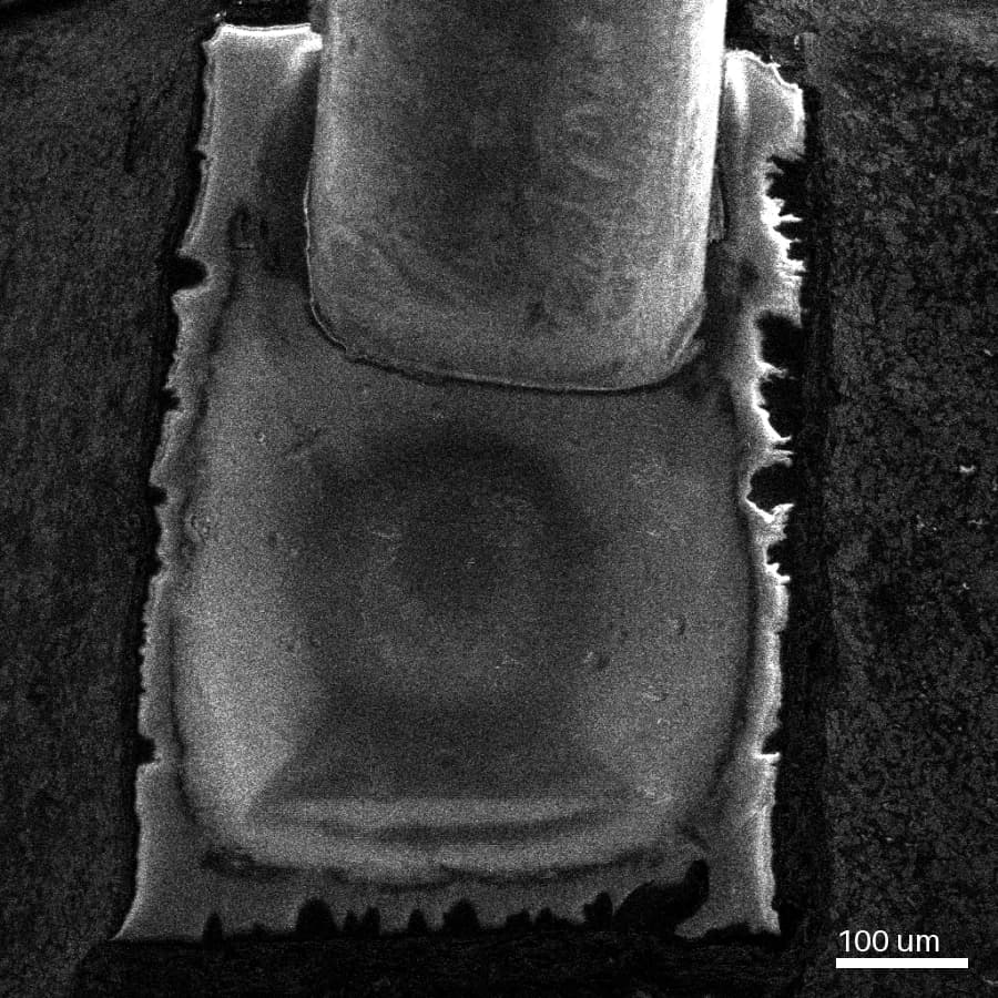
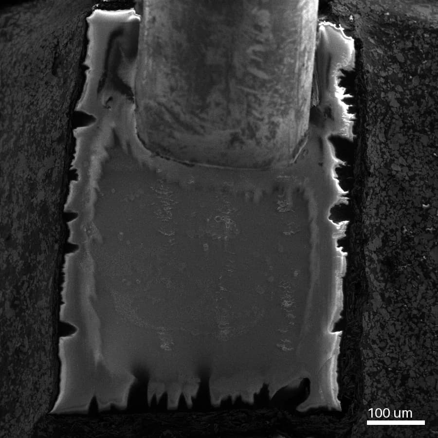
The Precision Charge Neutralisation (PCN) needle sits just above the block face throughout the acquisition, delivering gas over the imaged region to control charging. The collection field it creates is not uniform — signal falls off smoothly across each tile and across the mosaic — which is why the imagery in this report is flat-field corrected. The chamber pressure quoted above is measured away from this focused neutralisation region; locally, beneath the needle, it is considerably higher.

The PCN needle tip over the imaged region — The PCN needle tip (dark, top) over the imaged region, seen in a 399 µm preview frame.

The PCN needle over the block at a wider field of view (941 µm). It sits 15 µm above the sample surface and can return to the required XYZ position to sub-micron accuracy.

The needle and its gas footprint over the tile grid in Samurai — How Samurai sees it: the PCN needle (cyan) and its gas footprint (dashed circle) over the tile grid. The padlock marks tracking mode — the needle moves to keep the footprint centred on the tile being imaged.

The additive brightness and multiplicative contrast flat fields — The two flat fields applied to every tile — an additive brightness field (left) and a multiplicative contrast field (right). Each is derived by measuring the relative brightness and contrast respectively across all tiles in the dataset, removing outliers, averaging, and fitting a second-order polynomial.

The gas needle brought over the sample, with the live SEM view alongside: as the needle arrives, the charging artefacts collapse and the image stabilises (2× speed).

The gas switched off during tiling: charging noticeably increases once the gas flow passes below a certain threshold (~10× speed).

A mosaic captured across the whole block face, overlaid on the earlier low-dose overview beneath. The overview, taken without local gas, shows severe charging despite the low dose used; the higher-dose tiles captured with the gas footprint localised on each one are clean (43× speed).

Gas distribution visualised with secondary electrons — The whole block face is imaged with secondary electrons to clearly visualise the charging. The effective gas distribution on the sample surface, which is designed to form an under-expanded free jet (forward-peaked angular distribution), is clearly visualised at a low dwell time.

Charge drainage at a longer dwell time — Switching to a longer dwell time shows how the gas discharge can start to drain charge away from neighbouring areas below a certain gas-density threshold.

2. Sample behaviour in vacuum

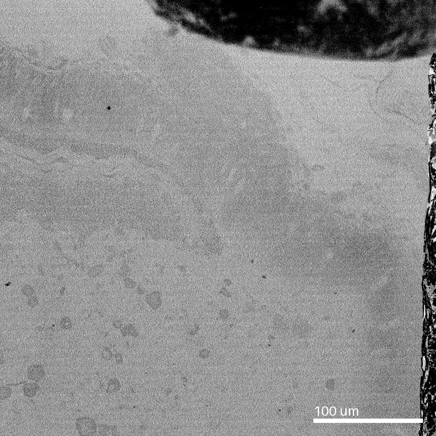
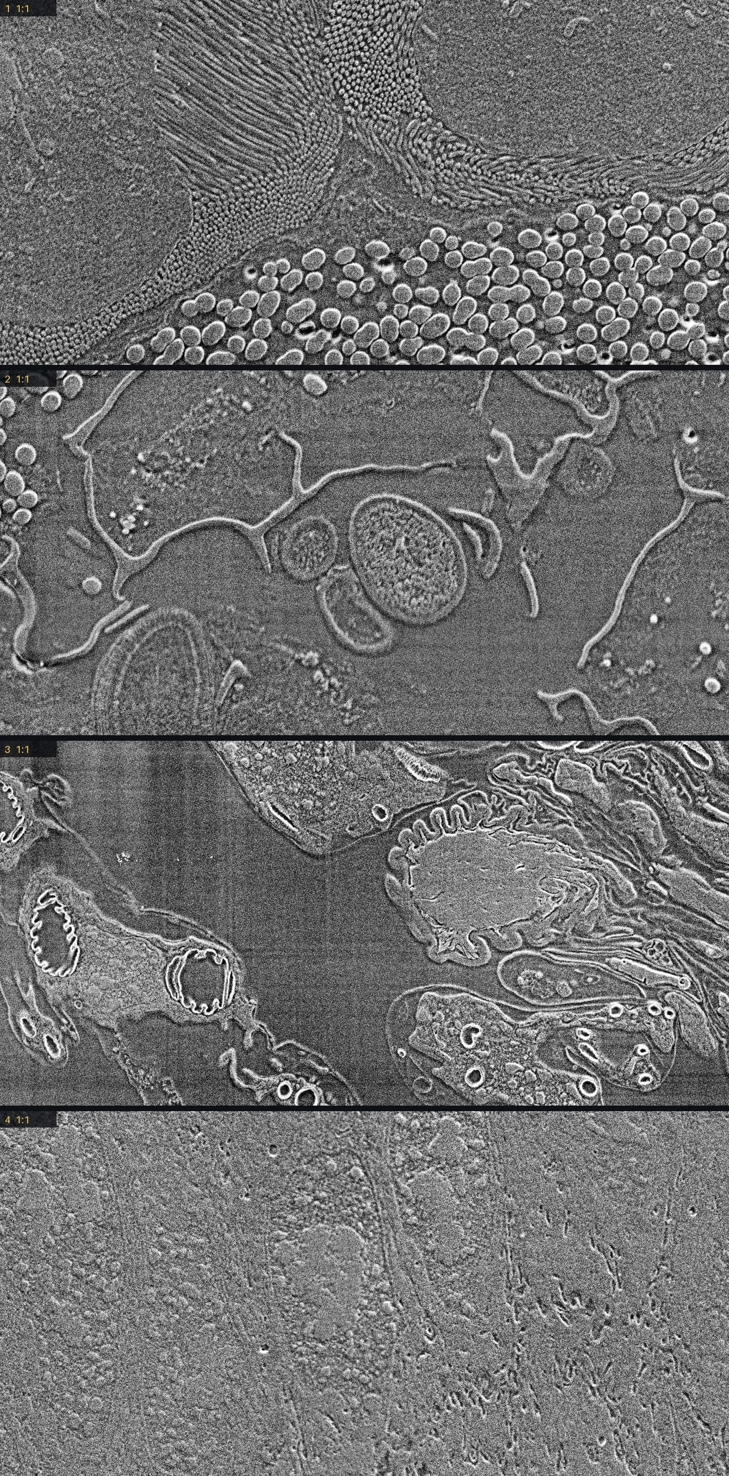
The cut surface imaged in secondary-electron mode 24 hours after the end of the acquisition: an 80-tile mosaic at 10 nm/px, 61,326×76,118 px (4.7 gigapixels), stitched with the same pipeline as the volume and shown here rebinned 2× to 20 nm/px. Acquired at 1.75 kV and 300 pA, 2.0 µs dwell, giving 37.5 e⁻/nm². Secondary electrons are far more sensitive to surface charge than the backscatter signal used for the volume, yet no charging is visible — Precision Charge Neutralisation holds the surface neutral. The noticeable topography indicates that the resin has shrunk slightly under vacuum. Press play to tour the surface at full resolution.

The full cut face (20 nm/px working image, 1.17 gigapixels). The tour zooms to the top-left corner at 50% sampling, pans diagonally across the face, and returns. Numbered outlines mark the 1:1 crops below. Scan striping was removed with a directional Fourier notch (horizontal and vertical, 1 deg tolerance) and local contrast equalised with CLAHE (511 px blocks, 256 bins, slope 1.6), applied across the whole gigapixel image.

Four 1:1 crops from the marked regions of the cut face — Four 1:1 crops from the marked regions, at full sampling.

3. Acquisition overview

A 938 µm survey view of the block face acquired mid-run. The knife-polished face of the block fills the frame; the dark speckled border is the silver paint on the sides of the block. The main mosaic and the high-resolution inset are outlined. Two further ROIs from the opening hours of the run were retired at cycle 13 and are not shown.

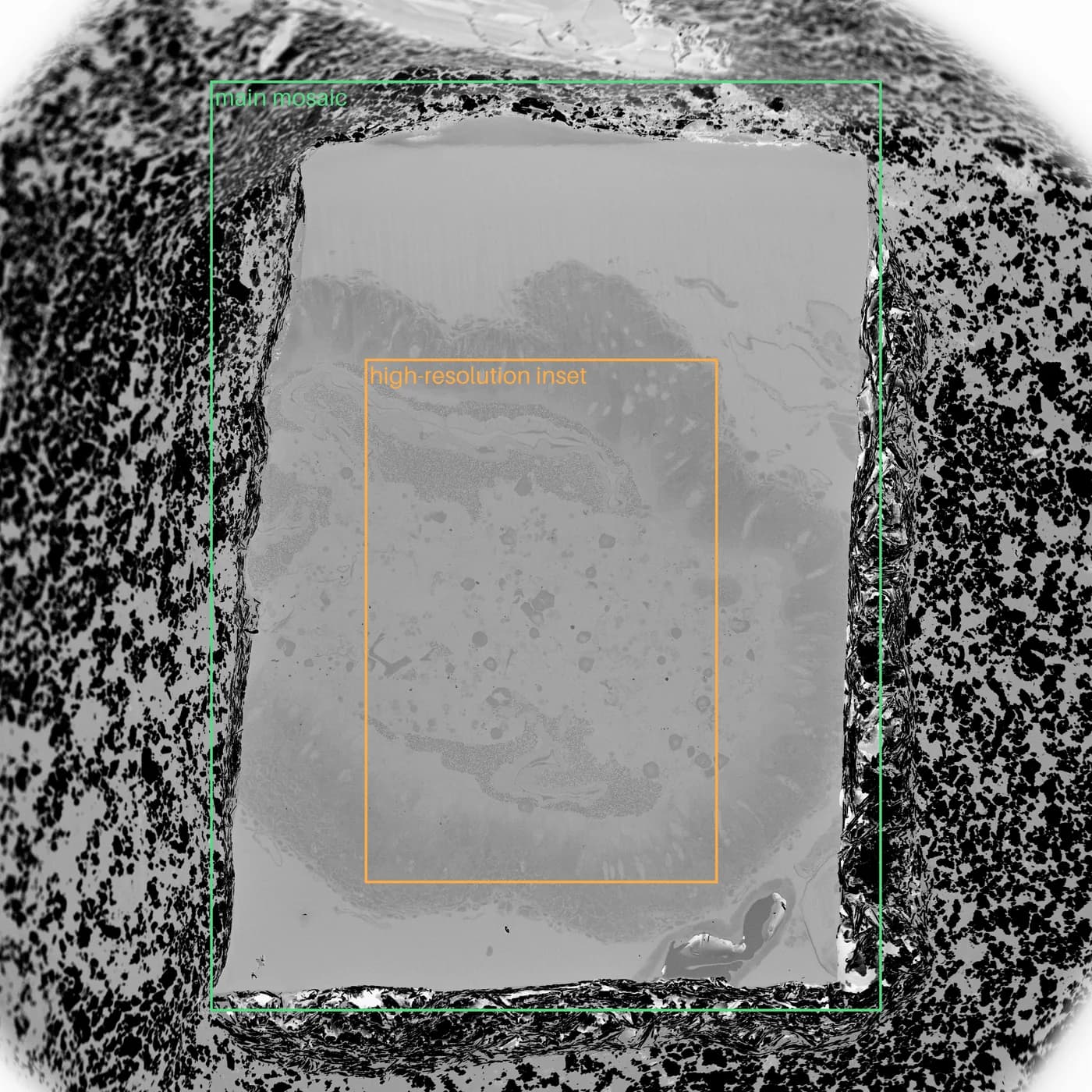
Block-face overview with ROI footprints — Block-face overview (229 nm/px preview capture). Footprints are drawn from stage coordinates after the mid-run frame corrections. The smooth interior is the freshly cut specimen surface; the silver paint around it provides conduction to ground.

ROI	Role	Tiles	Frame	Pixel	Cycles imaged	Images	Dose (e⁻/nm²)	Raw
ROI_3	main volume	35	4096²	32 nm	13–421 (170)	5,940	0.2–4.9	199.3 GB
ROI_4	high-res inset	2–6	8192²	10 nm	169–421 (253)	936	10–50	125.6 GB
ROI_1	opening survey (retired)	35	4096²	32 nm	1–13	405	0.2–0.7	13.6 GB
ROI_2	wide scout (one cycle)	11	1024²	150 nm	13	11	0.01	0.02 GB

4. The whole volume

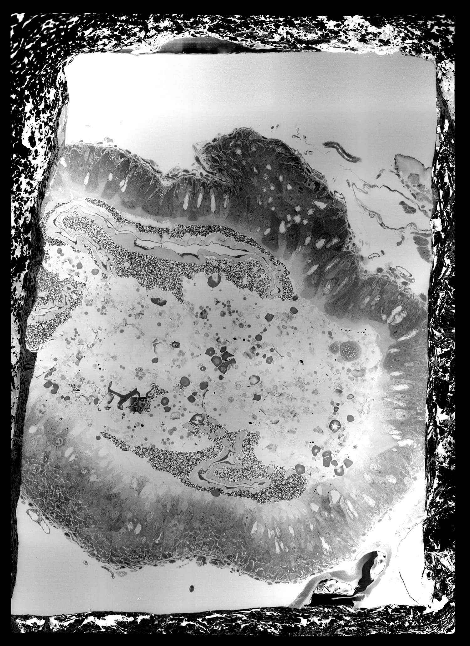
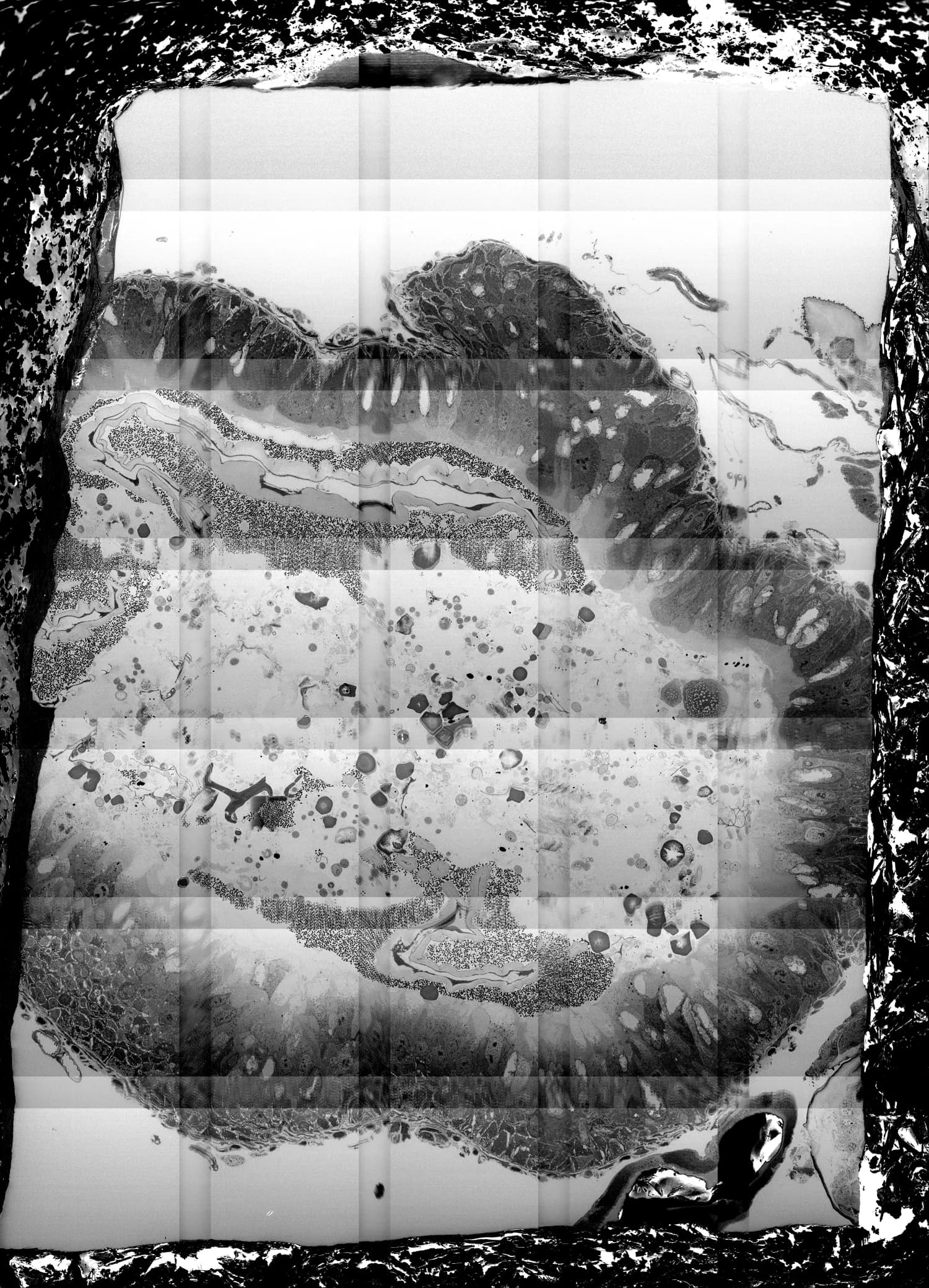
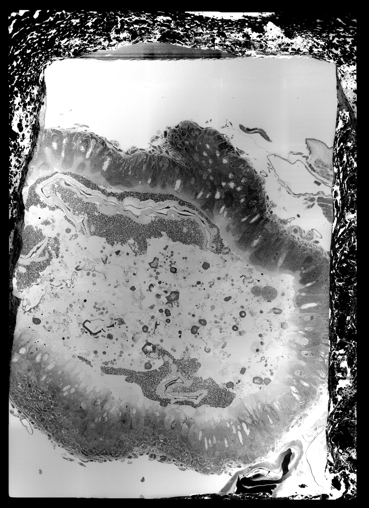
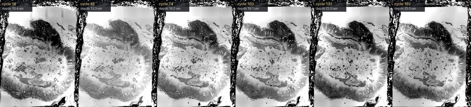
The full 35-tile mosaic — 577×817 µm per section — stitched, levelled and aligned through the dense run (cycles 13–164, 15.1 µm of depth), with sparse sections continuing to cycle 401.

The full 35-tile mosaic at cycle 100 — Cycle 100, the full 35-tile mosaic after flat-field correction, per-tile gain/offset levelling, systematic-misalignment correction, feather blending and illumination flattening. 128 nm/px working resolution from the 16-bit-faithful image pyramid.

The same cycle placed naively from stage coordinates — **Before:** the same cycle placed naively from stage coordinates with a single global tone window — tile patchwork, seams and the gas-field illumination gradient dominate.

Corrected mosaic at cycle 160 — **After** (shown at cycle 160): corrected and windowed on the specimen. Remaining tonal differences are real specimen structure.

The block face at six depths through the dense run.

Fly-through of the 152 dense sections, rendered from the full-resolution mosaics and scaled for display (850 nm/px). Tile placement is solved globally across the run, so tiles hold still from section to section rather than drifting against their neighbours.

5. The acquisition in motion

The acquisition was screen-recorded end to end. Below: a 41-hour unbroken stretch of the main run, compressed 2,958×. The PCN needle, in tracking mode, positions itself over each tile as it is captured, with the Katana Microtome advancing 100 nm per cycle.

Thu 06 Aug 22:40 → Sat 08 Aug, ~38 h at ×2,958 (60 fps, 1080p), ending as the stage is raised to focus. The wall clock is stamped bottom-left. The viewport's brightness visibly wanders through the run — a temperature-related detector drift that looks exaggerated here because the viewport uses a narrow display window; no image data was lost.

A later stage of the time lapse: five hours of acquiring selected high-resolution tiles with occasional background mosaics.

Setting up an acquisition: configuring the needle and gas footprint and the ROIs (2× speed).

6. Mid scale — a 2×2 tile block at 64 nm pixels

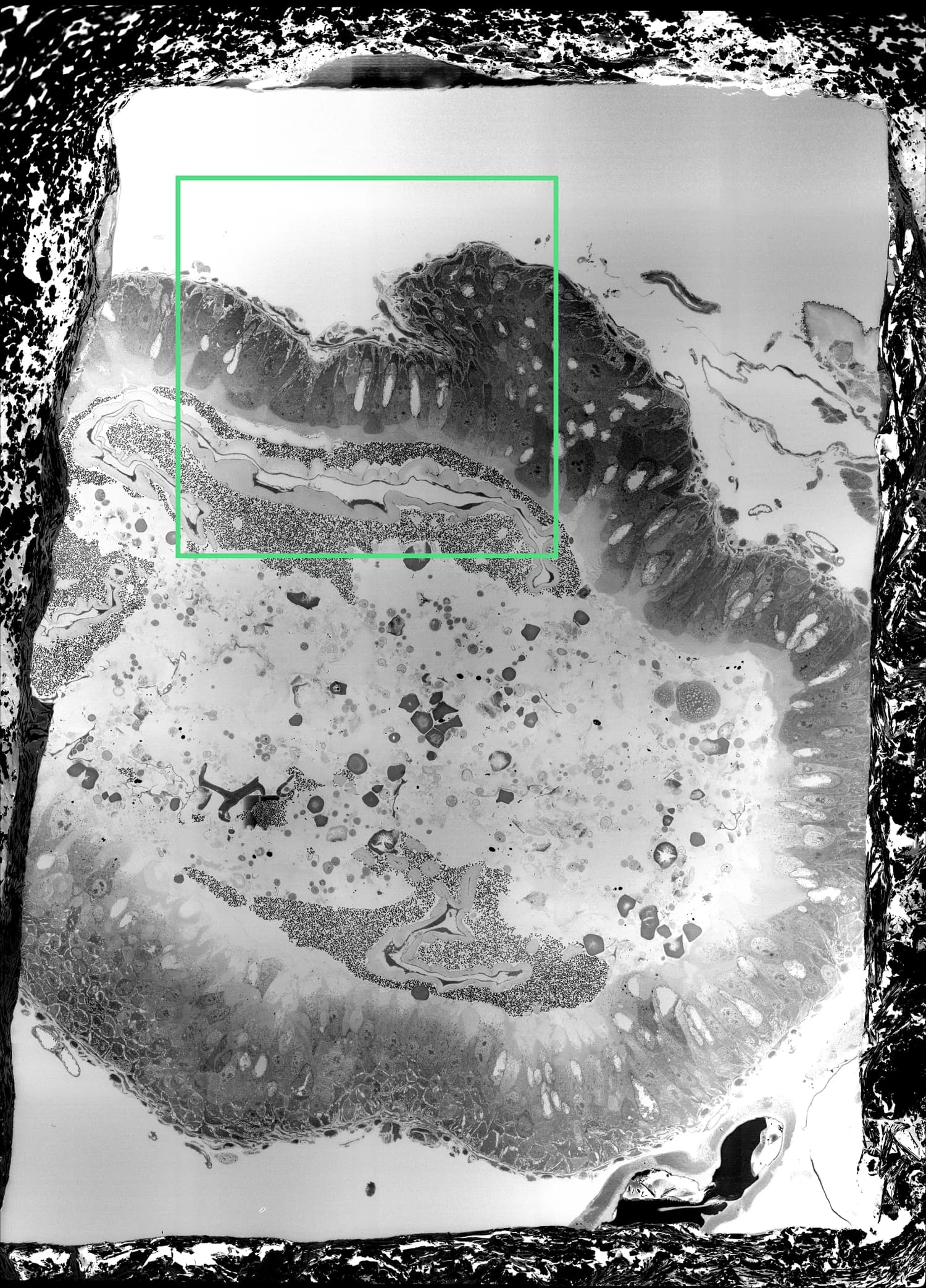
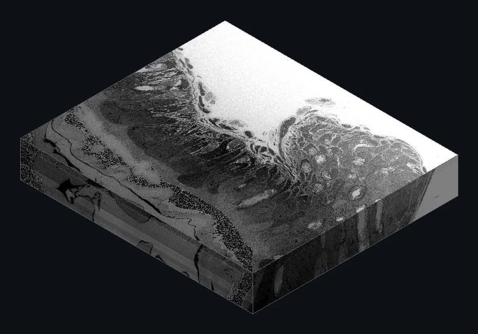
Four adjacent mosaic tiles rebuilt from the raw 16-bit frames at 2× binning — 64 nm pixels, 231×225 µm, 152 sections at 100 nm — near-isotropic voxels. Location within the mosaic shown first.

The 2x2 block located within the main mosaic — Within the main mosaic (cycle 100): the 2×2 block (green).

At a glance

Source	main mosaic, tiles D4-E5 (2×2)
Field	231 × 225 µm
Sections	152 at 100 nm (15.2 µm of depth)
Voxel	64 × 64 × 100 nm (2× binned)
Electron dose	4.9 e⁻/nm² (1.75 kV, 500 pA)
Volume	~790,000 µm³
Raw voxels sampled	10.2 G (4 tiles × 152 × 4096²)

Orthogonal planes through the block — press play and the cut lines sweep while the side panels re-slice live (60 fps). Depth axes are display-scaled (2× expanded for legibility); no pixel data is resampled in Z.

The mid-scale block rendered as a solid — The block as a solid: top face is a cut section, the sides are the resliced stack faces.

The clipping plane moves through the volume.

7. High resolution — 10 nm pixels

The high-resolution tile located within the main mosaic — Within the main mosaic (cycle 100): the high-resolution tile (orange).

At a glance

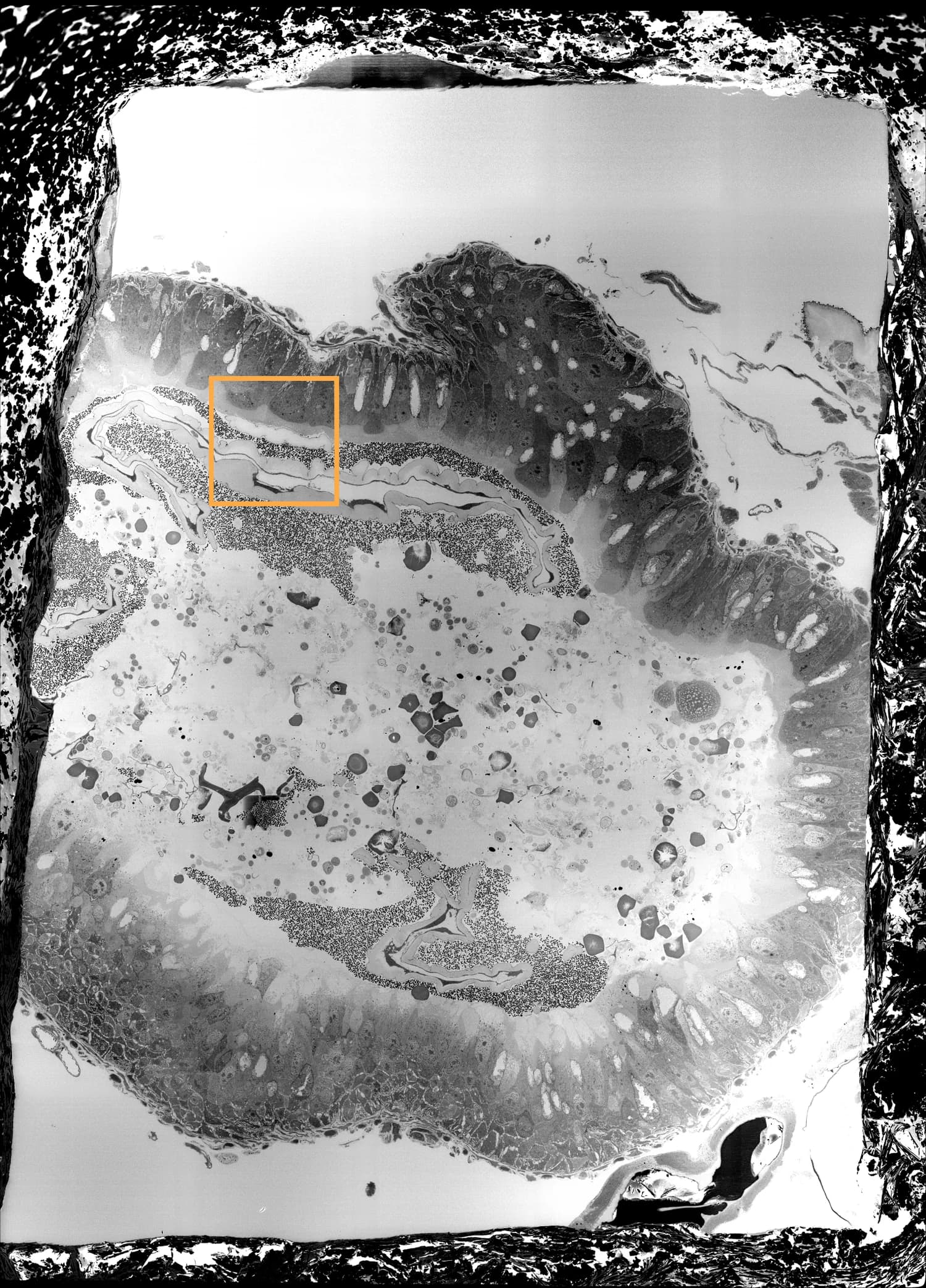
Source	high-resolution inset, tile C2
Field	70 × 57 µm (stable common region)
Sections	54 at 85 nm (4.6 µm of depth)
Voxel	20 × 20 × 85 nm (2× binned)
Electron dose	37.4 e⁻/nm² (1.75 kV, 500 pA)
Volume	~18,400 µm³
Raw voxels sampled	3.6 G (54 × 8192²)

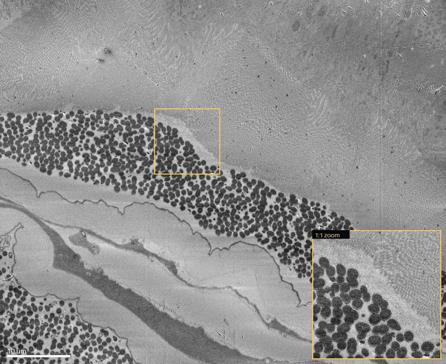
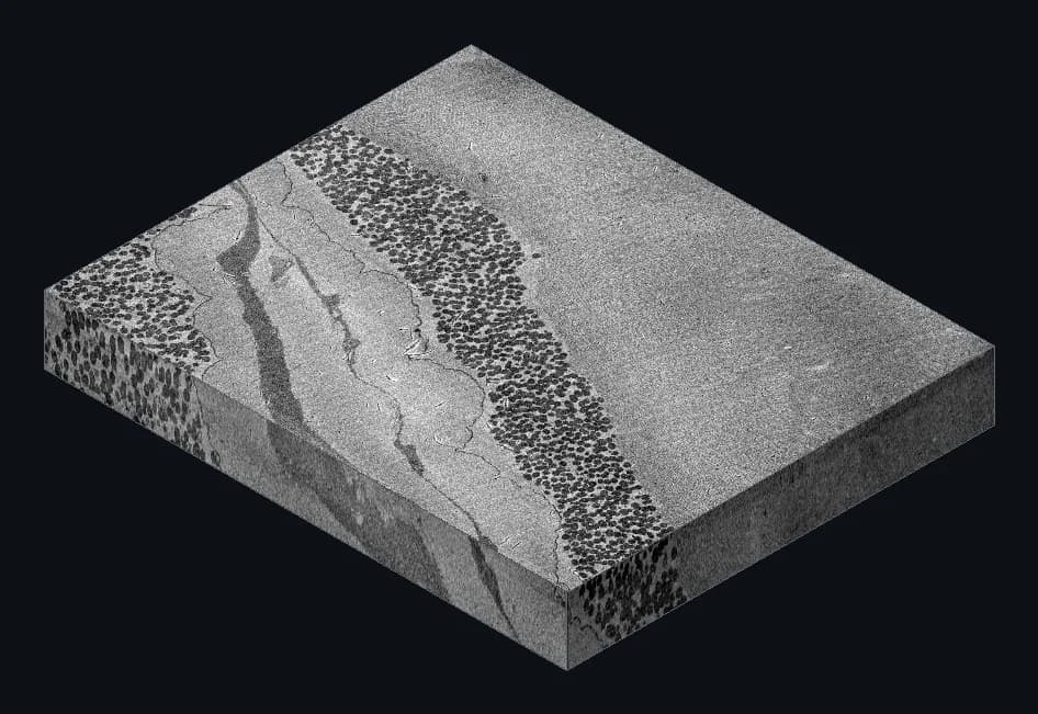
One tile of the high-resolution inset, 82×82 µm at 10 nm/px: cycles 252–305, 54 sections at 85 nm, registered and cropped to the common field (70×57 µm).

Cycle 278 at 20 nm/px with a 1:1-pixel inset of the granule band — Cycle 278, 20 nm/px working image with a 1:1-pixel inset of the granule band. The ellipsoidal bodies resolve cleanly. Above them the microvilli of the midgut brush border are visible; tracing individual microvilli would need slightly higher resolution, but there is sufficient detail to quantify properties such as their density and direction.

Orthogonal-plane view through the granule band — press play to sweep the cut planes (60 fps). Depth axes display-scaled 2×, no Z resampling.

The registered high-resolution sub-volume as a solid block — The registered sub-volume as a solid block.

The ellipsoidal bodies segmented by size-filtered thresholding, turning about the dataset's own Z axis like a turntable, seen from the same angle as the volume view, with the deepest section laid beneath as a floor.

8. Brightness: drift, corrections, reconstruction

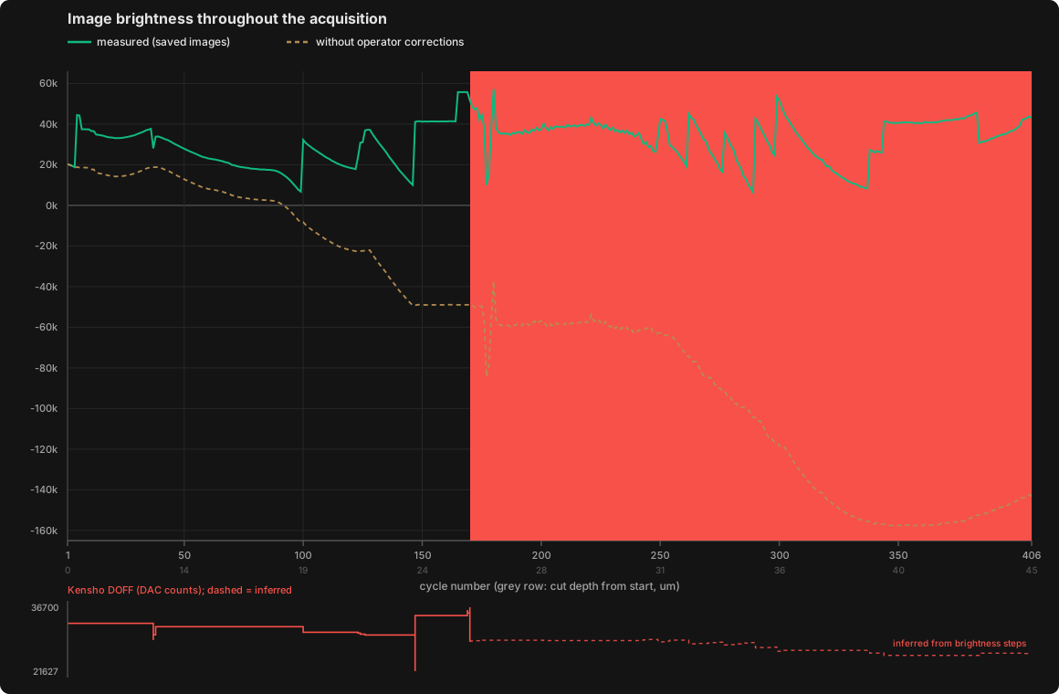
The Kensho detector's output drifted continuously downward through the run; the operator compensated by stepping the detector offset every few hours — the vertical transitions in the measured line. Aligning the data across those steps reconstructs the underlying drift: the dashed line shows how the brightness would have fallen with no corrections applied. The recorded offset commands calibrate the response at −29.1 DN per DAC count; where the logs carry no Kensho record (shaded), the offset trace is inferred from the brightness steps themselves.

Image brightness throughout the acquisition, measured against the reconstruction without operator corrections, with the Kensho detector offset trace beneath

9. Temperature throughout the acquisition

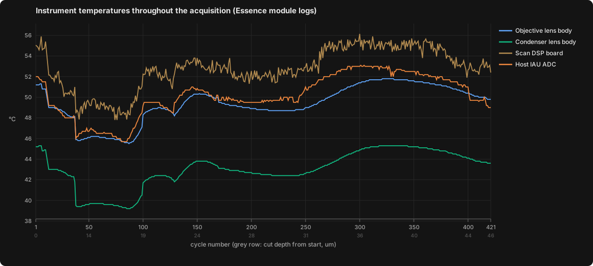
No environment sensor logged during this run, but the microscope's own module telemetry did: lens-body and electronics temperatures from the Essence service logs, joined to the acquisition via image timestamps. The sharp dip near cycle 127 is the idle period around the bridge stop; the excursions at the end accompany the vacuum-interlock outage.

Objective lens body, condenser lens body, scan DSP board and host IAU ADC temperatures across the acquisition

10. Geometry: drift and the tile-placement fingerprint

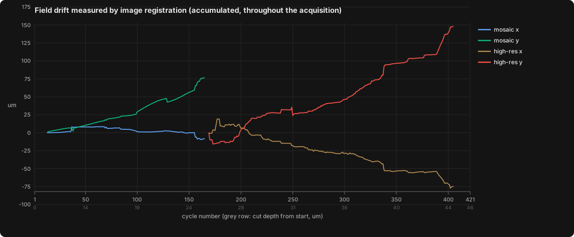
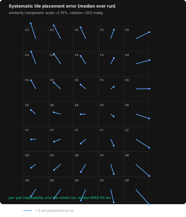
Registration measures how the imaged features moved — the accumulated trajectory already folds in the beam-shift recentring and calibration X/Y corrections the operator applied, so it represents how features would have wandered with no intervention. The field drifts by over 150 µm across the run and registration recovers it fully. Separately, the 35-tile grid carries a fixed placement fingerprint: a +2.1% scale and +0.2° rotation between stage and scan axes plus per-tile residuals, constant to 60 nm (median MAD) across the entire week.

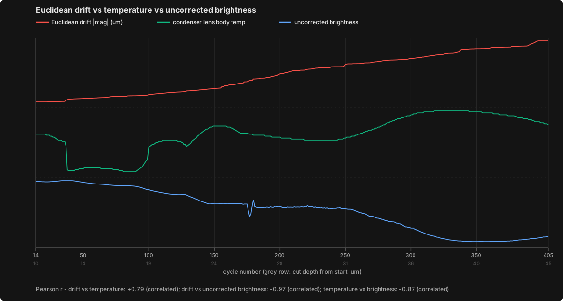
Accumulated field drift in x and y for the mosaic and the high-resolution inset, measured by image registration

Euclidean drift magnitude, condenser lens body temperature and uncorrected brightness plotted together across the run

The three slow envelopes move together: accumulated drift tracks the column's thermal state (r = +0.79 against the condenser lens body), and the uncorrected detector brightness falls as both rise (r = −0.97 against drift, −0.87 against temperature) — consistent with a common thermal origin.

Systematic tile placement error across the 35-tile grid, with a similarity component of +2.10% scale and +203 mdeg rotation

Processing summary

Step	Method
Tile placement	stage grid + fixed per-tile offsets (NCC on overlap strips, 13 cycles sampled)
Flat fields	per-cycle brightness + contrast fields from the tile stack, smoothed to 25% of tile size
Tile levelling	per-cycle gain + offset solve from overlap medians (content cancels)
Tile placement	global least-squares solve over every tile in every cycle: overlap offsets within a section, the same tile in the sections either side, and a smoothness term through depth, so a section whose overlap measurement fails takes its placement from its neighbours rather than jumping. Stage steps part-way through a cycle are corrected from their own measurements
Illumination	robust 2nd-order polynomial flatten per section (gas-field gradient)
Outlier guard	49 of 5,425 suboptimal tiles interpolated for cosmetic appearance (for example a tile manually skipped, or a brightness or contrast change made midway through tile acquisition). Four of those were absent from the capture altogether and were taken from the adjacent cycle
Debris	no significant debris requiring tile reacquisition anywhere in the dataset
Section registration	bandpassed phase correlation, consecutive + skip-one repair
Brightness over Z	chained percentile matching between consecutive sections
Stripe removal	a light FFT notch filter on low-level horizontal scan noise
Z axis	never resampled; section spacing applied at display time only

11. Run record

Cycle	Event
1	Run start 2026-08-03 20:32 — ROI_1 survey, 100 nm sections, 2.2 kV / 150 pA
13	Reframe: ROI_1 retired; ROI_3 becomes the main 35-tile mosaic
36–37	Beam to 1.75 kV / 500 pA; ROI_3 dwell settles at 0.4 µs × 2-line averaging
127	Stopped and resumed after an SEM bridge reconnect
164–168	Stopped; beam cycled and imaging conditions re-established
169	Reconfiguration: ROI_4 8192²/10 nm inset added; ROI_3 to every 20th cycle; 70 nm sections
249	Stopped and re-locked; 85 nm sections; high-resolution inset grows to 4 tiles (later 6)
406	Vacuum interlock triggered by a 90 ms pressure blip; imaging paused 2 h 35 m and the affected images excluded
421	Last images 2026-08-10 08:54; run stopped at operator's console

Spod5 — acquired 2026-08-03 → 2026-08-10 on Samurai 3 / TESCAN CLARA. Video in this edition is compressed for distribution; full-resolution masters are held separately. Report revised 2026-08-18.